e-puck robot
Back to Work
Presented at ALIFE 2025 · Kyoto / Online
Evolutionary Robotics · Hebbian Learning

Post-Evolution Adaptation

Code

Research Team

Supervisor Talal Shaikh
Lead Author Hamze Hammami
Member Eva Denisa Barbulescu
Member Mouayad Aldada
Member Muhammad Saad Munawar
Scroll
The Problem

Genetic Memory,
No Lifetime Learning

The Limitation

Genetic controllers are effective at optimising behaviour in fixed environments, but they encode only what evolution has seen. Even small changes at deployment can cause failure, and covering every possible scenario through evolution alone is computationally expensive and impractical.

  • Limited to generational experience, not runtime adaptation.
  • Brittle under sudden environmental changes.
  • Retraining from scratch is costly for each new scenario.
The Proposal

Separate genetic memory from lifetime learning. Keep the evolved genome as a fixed foundation, then apply Hebbian plasticity on top, adapting weights on-the-fly without touching the core knowledge.

  • Adapt the genotype to novel situations at runtime.
  • Preserve core knowledge, reset after each trial.
  • Zero-shot: weights develop only from neuron co-activation during the robot's lifetime.
Figures, add images below
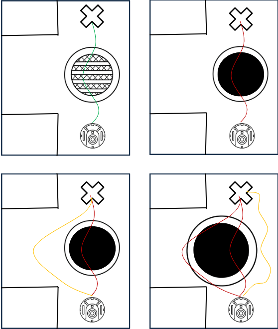
Robot trajectories: GA vs Hebbian

Robot trajectories comparing GA-only vs Hebbian-adapted controllers under base and changed environments. Top row: GA alone. Bottom row: post-evolution Hebbian adaptation.

Genetic Algorithm

Fitness Function

A dual fitness system combining behaviour fitness and a goal reward. The behaviour components penalise spinning and collision while rewarding forward motion and correct junction turns. The goal reward scales with Euclidean distance to the target position.

Forward Motion
forwardFitness = (vleft + vright) / 1.5

Rewards the robot for moving forward. Clamped to [0, 1], negative values (reversing) are treated as zero.

Forward fitness
Collision Avoidance
avoidCollisionFitness = 1 − (max(proximitySensors))3

Penalises proximity to obstacles. The cubic exponent gives a sharper penalty as the robot gets closer, given double weight in the combined score.

Collision avoidance fitness
Anti-Spinning
spinningFitness = 1 − |vright − vleft| / 2

Penalises large velocity differences between wheels. Discourages in-place spinning behaviour that wastes time without progress.

Spinning fitness
Junction Decision
junctionFitness = 1 if correct turn, 0 otherwise

Binary reward at the T-junction. The robot must turn right when light is present and left when absent, the core behavioural objective of the task.

Junction fitness
Goal Reward
dist = √((xg−x)² + (zg−z)²)  ·  reward = 1 − min(1, (1.7 × dist)³)

Distance-based reward scaling the robot's proximity to the target position. A cubic scaling makes the reward drop off steeply with distance.

Goal reward
Combined Behaviour Fitness
combinedFitness = (fforw + 2·favoid + fspin + fjunction) / 5

Weighted combination of all four behaviour components. Collision avoidance is given double weight to prioritise safe navigation above all else.

Final Fitness
finalFitness = (combinedFitness + reward) / 2

The average of behaviour fitness and goal reward. Balances the quality of movement with whether the robot actually reaches its target.

Base Environment

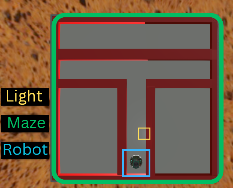
The T-Maze

A T-shaped maze serves as the training and testing environment for the genome's observable states through Hebbian learning. The robot starts at the base of the T, with a light source that appears or disappears depending on the task.

The robot must learn to turn right at the junction when light is present, and left when light is absent. This rule is not hardcoded; it must emerge from the fitness landscape during evolution, and then be preserved or adapted through Hebbian plasticity at runtime.

T-shaped maze base environment

Base environment in Webots. The robot (blue) starts at the T's base. The light source (yellow) determines which direction it must turn at the junction.

Phase 1

Genetic Training

The first phase trains a controller through a standard genetic algorithm. The T-maze environment serves as the foundation to evolve an optimal genome for the navigation task. This ensures a solid baseline controller is established before any plasticity is applied.

Evolution Process
Optimal Gene
The Problem in Practice

Genetic Failure

When the environment changes, even slight modifications can cause the evolved controller to fail. The genome was never trained in the altered environment, and training for every possible variation is computationally expensive. Reusing examples of the same situation can also introduce bias through environmental imbalance.

Two Obstacles
Four Obstacles
Hebbian Learning

Neuromodulation Signal

Neuromodulation is the process of altering nerve activity to normalise nervous system behaviour. Here, the Hebbian learning rate is adaptively scaled using the robot's current fitness as a continuous guiding signal.

Ne = N × max(0.2, F)
N, base Hebbian rate (maximum) Ne, effective rate applied to weight updates F, current fitness value

The equation scales the maximum signal based on fitness. The max function ensures the rate never drops below 0.2, preventing zero modulation. A robot performing poorly still adapts slowly; a robot performing well strengthens connections faster.

Neuromodulation signal
Low Fitness · F = 0.1
max(0.2, 0.1) = 0.2 Ne = 0.002 × 0.2 Ne = 0.0004
High Fitness · F = 0.9
max(0.2, 0.9) = 0.9 Ne = 0.002 × 0.9 Ne = 0.0018
Mechanism

Hebbian Synaptic Adaptation

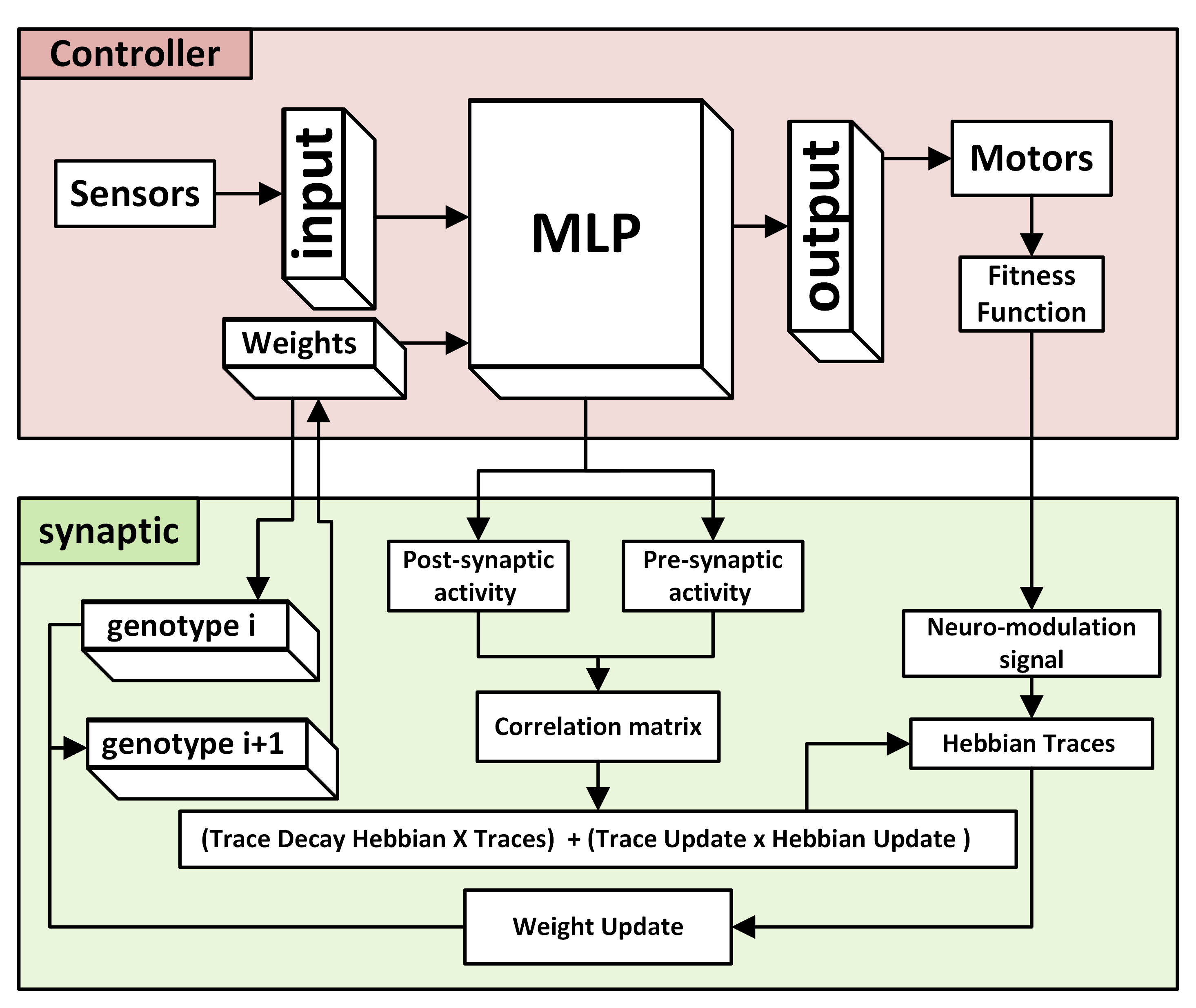
Pre- and post-synaptic activations form a correlation matrix that drives Hebbian trace updates. Raw Hebbian updates can cause unstable weight growth, so a trace decay mechanism discards older correlations to prevent runaway growth.

Traces A temporal history of neural co-activations. The neuromodulation signal scales these traces to produce the final weight update.
Decay Retains 95% of the previous trace while integrating 5% new correlation data, preventing old patterns from dominating.
Clipping Weights are clipped to ±Wmax after each update to prevent saturation or collapse.
Decay Ti+1 = (Tdecay × Ti) + (Tupdate × C)
Scaling ΔW = Ne × Ti+1
Update WT+1 = WT + ΔW
Clipping WT+1 = clip(WT+1, −Wmax, Wmax)
Hebbian synaptic adaptation diagram
Phase 2 · Lifetime Learning

Hebbian Adaptation in Action

With the evolved genome loaded, Hebbian plasticity activates at runtime. The robot encounters the obstacles it previously failed at, and its synaptic weights begin adapting on-the-fly. The network visualisation shows weight changes as they happen: small flashes indicate minor adjustments, green flashes mark significant positive reinforcement of successful pathways, and orange marks significant negative changes weakening unhelpful connections.

Phenotypic Changes · Live Network
Positive weight Negative weight Strengthening Weakening
Small changes
Hebbian Success

Zero-Shot Adaptation to Unseen Environments

Hebbian plasticity lets the robot successfully complete the task on the first attempt in environments it has never trained in. By creating a new observable state of the genome within the same lifetime, without rewriting a new generation, the same code solves both obstacle configurations.

Two Obstacles
Four Obstacles
Experimental Results

Performance Comparison

The experiments compare the GA-only controller against the Hebbian-adapted controller across three environments: the base training environment, and two unseen obstacle configurations. Key measures are task success, time to reach the goal, path length, speed, position error, and average weight change magnitude.

Worth noting: the GA controller did avoid some obstacles in certain runs. This is part of how the genetic algorithm works, the evolved behaviour can sometimes generalise partially to new situations. However it is not predictable or reliable. The Hebbian controller, adapting a live network on the same fitness signal it was trained on, performs more consistently, but this does not guarantee 100% success in all cases either. The improvement is real but the system is still probabilistic.

GA Only · Genetic Algorithm Controller
Base GA 2 Obstacles GA 4 Obstacles GA
LeftRight LeftRight LeftRight
Success (0/1)110000
Time-to-Goal (s)213.82174.62FailedFailedFailedFailed
Path Length (m)0.91140.88540.61950.72980.61900.5520
Average Speed (m/s)0.00360.00350.00250.00290.00250.0022
Final Position Error0.02210.03190.25920.12250.25920.3428
Hebbian · Post-Evolution Adapted Controller
Base Hebbian 2 Obstacles Hebbian 4 Obstacles Hebbian
LeftRight LeftRight LeftRight
Success (0/1)111111
Time-to-Goal (s)192.32156.77192.29156.48191.26161.25
Path Length (m)0.89150.88280.89150.88360.88930.8813
Average Speed (m/s)0.00360.00350.00360.00350.00360.0035
Final Position Error0.02330.03270.02320.03270.02330.0327
Weight Change Mean2.97022.59063.01322.61653.11062.6973

Brain Activity Feedback

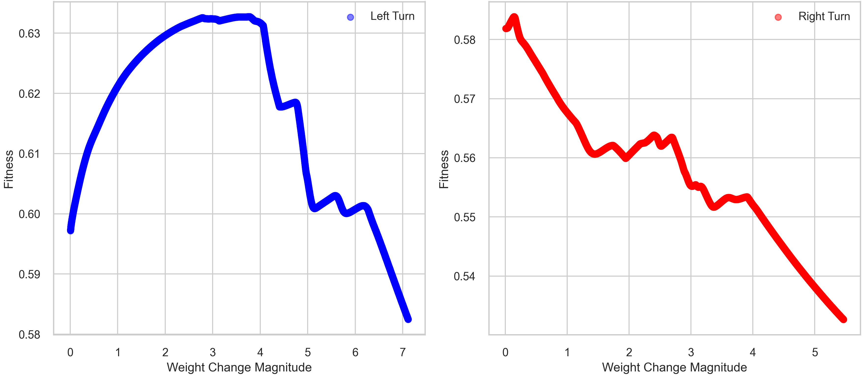
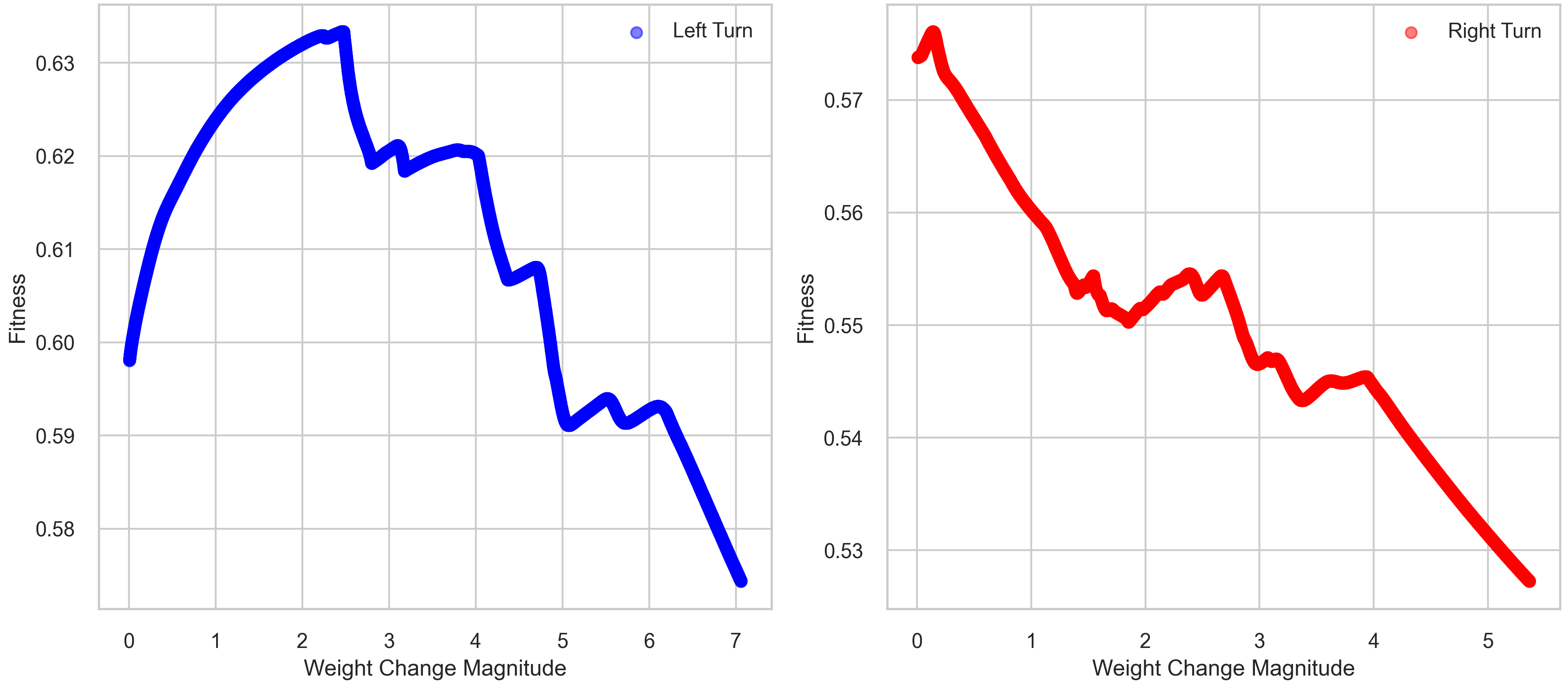
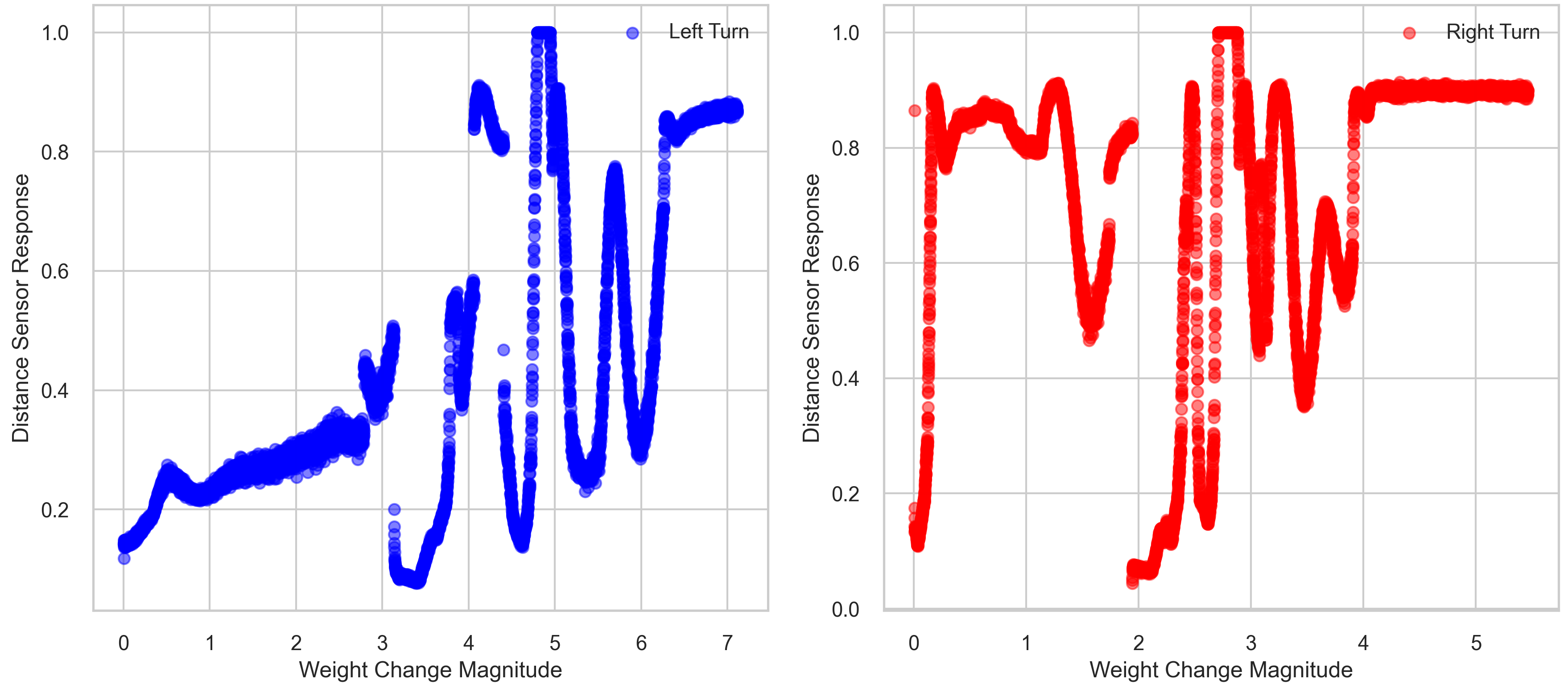
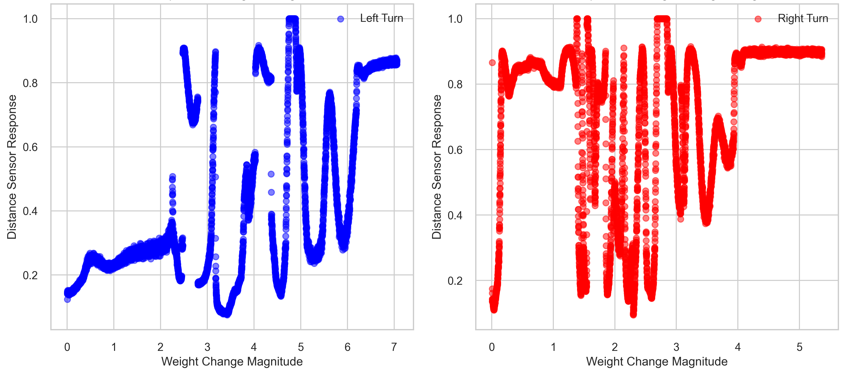
Each plot shows how weight change magnitude correlates with fitness and distance sensor response across different runs. The pattern of weight changes reflects the robot actively adapting its synaptic connections in response to its environment. More obstacles produce more weight activity, confirming the Hebbian mechanism is responding to environmental complexity rather than noise.

2 Obstacles · Fitness vs Weight Change 2 obstacles fitness vs weight change
4 Obstacles · Fitness vs Weight Change 4 obstacles fitness vs weight change
2 Obstacles · Distance Response vs Weight Change 2 obstacles distance response vs weight change
4 Obstacles · Distance Response vs Weight Change 4 obstacles distance response vs weight change
Experiment 2

Light Experiment

The same genome trained in a high-luminosity environment is then deployed in a low-light setting. The altered light sensor readings cause the genetic controller to fail at the junction task. Hebbian plasticity adapts the synaptic weights on-the-fly, recovering the correct behaviour without any retraining.

Since this experiment involves more persistent environmental changes rather than physical obstacles, a higher adaptation scale was needed. A higher Hebbian learning rate allows the network to respond more quickly to the shifted light distribution, but at the cost of more erratic and less controlled behaviour.

High Light · Trained Environment
Low Light · Gene Fails
Low Light · Hebbian Recovers
Discussion

Implications

The results sit at the intersection of evolutionary robotics and biological learning theory. Several broader implications emerge from the architecture, each grounded in how biological systems separate memory from adaptation.

Biological Parallel

The Baldwin Effect

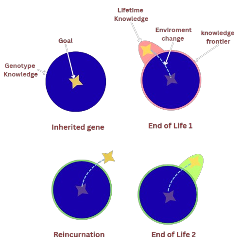
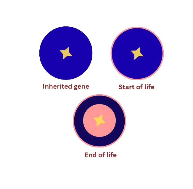
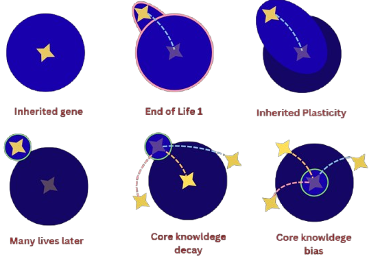
Starting with a fixed genotype at birth, the robot performs its task within a lifetime of Hebbian learning. This raises performance without changing the inherited genotype, reacting to what the initial gene cannot resolve. When the genome is passed to the next generation it does not inherit the plasticity changes. The lifetime reset prevents genetic assimilation, keeping the core memory clean and generalisable.

Baldwin effect diagram
Non-changing benefits diagram
Stable Environments

Non-Changing Benefits

The benefit of Hebbian adaptation is not limited to environmental change. Even in stable environments, it can temporarily make the initial gene more optimal. However the plasticity changes are still not saved post-reincarnation, even if they improve performance. Preserving them would accumulate bias over generations, degrading the generality of the core genome.

Memory Integrity

Benefits of Reincarnation Reset

If offspring inherit plasticity changes, over generations a bias toward specific environmental changes accumulates. The reset ensures core knowledge stays intact and remains adaptable. It also prevents the genome from becoming overfitted to a single environment, keeping it light enough for zero-shot adaptation wherever it is deployed.

Reincarnation reset diagram

Limitations

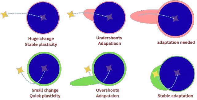
The current implementation uses a static maximum Hebbian learning rate, manually tuned per experiment. Neuromodulation already scales learning using fitness, but it is missing the environmental magnitude of change as a signal. A large rate in an already-familiar environment causes overreaction. A rate too small for a large environmental shift means the robot adapts too slowly within the trial.

Environmental feedback limitations diagram
Current Gap The system detects performance drop via fitness but not the degree of environmental novelty. The ideal system would sense how much the environment has changed and scale N accordingly.
Future Direction Future work aims to detect context shifts by streaming sensory data through a spike-dependent network, allowing N to adapt from the base Hebbian rate to environment-sensitive rates dynamically.
Network Scale Experiments used a simple MLP with low-dimensional input. Future implementations will test more complex sensory data such as point clouds or LiDAR while retaining the same plasticity mechanism.
Generalisation All experiments use a single e-puck in a T-maze. The approach needs to be validated on different platforms including drones and legged robots across more complex terrains.